Deep Learning
Universes that Learn: Cellular Automata Applications and Acceleration
November 4, 2020
19 min read


For people with passing familiarity with the idea of cellular automata (CA), the first thing that comes to mind is probably John Horton Conway’s Game of Life. After Martin Gardner described Conway’s Game of Life (often abbreviated to Life, GOL, or similar) in his mathematical games column of Scientific American in 1970, the game developed into its own niche, attracting formal research and casual tinkering alike. With a significant population of dedicated hobbyists as well as researchers, it wasn’t long before people discovered and invented all sorts of dynamic machines implemented in the GOL. These can be quite complicated and include universal computers, some that can self-replicate. Other famous CA include Stephen Woflram’s Rule 110, proven to be Turing complete, capable of universal computation by Matthew Cook in 1998.
While Conway’s GOL is the most famous set of CA rules, the concept seems to have origins in conversations between John Von Neumann and Stanislaw Ulam in the 1940s when they both worked at Los Alamos National Laboratory. This eventually yielded a 29-state CA system which laid the foundations for Von Neumann’s universal constructor, a machine that operates in Neumann’s CA world and can make identical copies of itself.
Cellular automata can be generally described as a collection of cells, each with a state or states that change according to some rules based on each cell’s local context. Although cells are often arranged in rectangular 2D grids, the arrangement can be arbitrary, and while states are most often discrete, rules and states can also be continuously valued and even differentiable (more on that later). Many of the most interesting CA universes bear a striking resemblance to physical phenomena such as growth, diffusion, and flow, and CA have been described as the computer scientist’s discretized version of the physicist’s concept of fields. They are often used as the basis for physics models, and at least one prominent researcher thinks the resemblance is more than superficial.
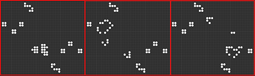
A glider generating pattern known as a Simkin glider gun. Here two “fish hooks,” stable patterns that destroy incident cells, consume the gliders before they travel to the edge of the grid. This example was simulated in Golly.
There has been significant research enthusiasm for CA beginning in the 1960s, and the field has seen steady growth in the number of papers published each year. They’ve been used to model everything from chemical reactions and diffusion, to turbulence, to epidemiology, and they are a cornerstone of fundamental complexity research. Given the visual similarity to a wide range of natural phenomena (remember, GOL rules were developed specifically to mimic life-like characteristics of growth and self-organization), it’s not surprising that CA have found so many applications in modeling and simulation. As mentioned above, cellular automata rules can often result in systems capable of universal computation, i.e. they can compute any algorithm that can be programmed. This holds true for the exceedingly simple 1D Rule 110 all the way up to the comparatively complicated 29-state Von Neumann system.
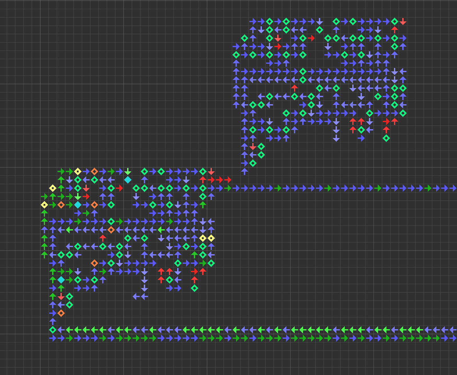
A small self-replicating constructor in Von Neumann’s CA universe. The constructor has built a copy of itself and is now copying the instruction sequence (the mostly blue line of arrows trailing off to the right) for the new machine. This example was simulated in Golly.
We’ve also seen both Turing complete computers and self-replicating universal constructors implemented in CA universes. Somewhat counterintuitively, Turing completeness is surprisingly easy to stumble upon by accident when building any system of sufficient complexity. However, we want to build not only computational systems but intelligent ones as well. We know they can compute, but can they learn?
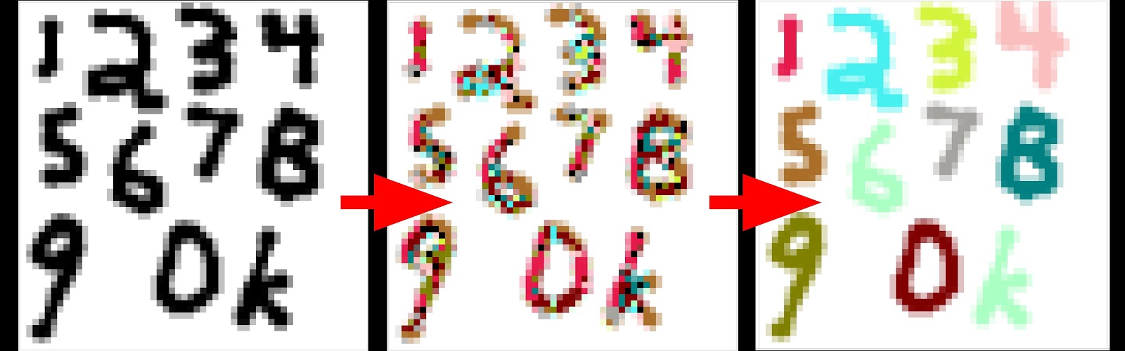
Demonstration of “Self-classifying MNIST Digits.” The digits all start out as a single color and over time the cells build a consensus classification of each digit, represented by color. The attentive reader may also point out that multiple digits are classified, and indeed this occurs simultaneously (the image is not a collage of separate samples), suggesting the possibility of cellular automatic image segmentation. The image is a screenshot of the interactive figure CC BY SA Randasso et al. https://distill.pub/2020/selforg/mnist/.
The interactive machine learning journal Distill.pub has a nascent research thread: “differentiable self-organizing systems.” They’ve only published two articles in this thread so far: a demonstration of self-generating and self-repairing graphical sprites, and self-classifying MNIST digits. Both articles are built around interactive visualizations and demonstrations with code, which is well worth a look for machine learning and cellular automata enthusiasts alike.
Interested in getting faster results with deep learning?
Learn more about Exxact workstations for AI research starting at $3,700
In the MNIST article, repeated application of CA rules eventually cause the cells to settle on a consensus classification (designated by color) for a given starting digit. Applying n updates to an image according to a set of CA rules is not altogether dissimilar to feeding that same image through an n-layer convolutional network, and so it is not surprising that one can use CA to solve a classic conv-net demo problem. In fact, as we’ll see later, CA rules can be implemented effectively as convolutions which means we can take advantage of the substantial development efforts in software, hardware, and systems for deep learning.
CA can do a lot more than “just” simulate physics, however the nature of CA computation doesn’t lend itself to conventional, serial computation on Von Neumann style architectures. To get good performance high-throughput parallelism is required. Luckily, while bespoke, single-purpose accelerators may offer some benefits, we don’t need to develop new accelerators from scratch. We can use many of the same software and hardware tools used to accelerate deep learning to get similar speedups with cellular automata universes.
It’s useful to keep in mind that Von Neumann developed his 29-state CA using pen and paper, while Conway developed the 2-state GOL by playing with the stones and grid on a Go board. While it would probably be comparatively simple to use a computational search to discover new rules that satisfy the growth-like characteristics Conway was going for in Life, the simple tools used by Neumann and Conway in their work on cellular automata are a nice reminder that Moore’s law is not responsible for every inch of progress.
CA systems, like neural networks, are not particularly well-suited to implementation on typical general purpose computers. These tend to be based on the Von Neumann architecture (although multiple cores and cache memory do stretch the original concept), compute instructions sequentially, and emphasize low latency over parallelism. A cellular automaton universe, on the other hand, is inherently parallel and often massively so. Each individual cell must make identical computations based only on its local context.
The utility of CA systems led to several projects for dedicated CA processors, much like modern interest in deep learning has motivated the development of numerous neural coprocessors and dedicated accelerators. The specialized computers are sometimes called cellular automata machines (CAMs ). In the 1980s and 1990s CAMs were likely to be custom-designed for specific, often one-off purposes. The CAM-brain was an attempt to build a system using a Field Programmable Gate Array (FPGA) to evolve CA structures in order to simulate neurons and neural circuits. Systolic arrays, basically a mosaic of small processors that transform and transport data from and to one another, would seem to be an ideal substrate for implementing CA and indeed there have been several projects (including Google’s TPU) to take this approach. Systolic arrays sidestep one of the most often overlooked hurdles in high-performance computing, that of communications bottlenecks (the motivation behind Nvidia’s NVLink for multi-GPU systems and AMD’s Infinity Fabric.
There have also been algorithmic speed-ups for the most popular CA rules: Hashlife, developed by Bill Gosper in the 1980s, uses memorization to speed up CA computations by remembering previously seen patterns. Just like special purpose accelerators for deep learning (e.g. Graphcore’s IPU or Cerebras’ massive wafer-scale accelerator), single-purpose accelerators for CA computations trade flexibility for speed.
Notable projects for building CA acceleration hardware include the cellular automata machine (CAM) by Norman Margolus and Tommasso Toffoli, which underwent several iterations in the 1980s. The first CAM prototype, described in 1984, could update a grid of 256 by 256 cells at a rate of 60 frames per second, in other words computing nearly 4 million updates a second. This was about a thousand times faster than execution on a comparable general purpose computer at the time. The speed-up was largely accomplished by mapping CA rules to memory and scanning over the grid rather than genuine parallelization. For comparison, the GPU PyTorch implementation in the next section updates more than 128 million cells each second on a personal workstation.
The supercomputer company Thinking Machines also devoted substantial efforts to building a massively parallel architecture for scientific computing. The so-called Connection Machine line of supercomputers were built with thousands of parallel processors arranged in a fashion akin to CA, but they were hardly the sort of computer one might purchase on a whim. The CA-based architecture made Connection Machines well-suited for many challenging scientific computing problems, but the company filed for bankruptcy in 1994.
Another project specifically for simulating neuronal circuits in CA (with the goal of efficiently controlling a robotic cat) was the CAM-brain project spearheaded by Hugo De Garis. The project went on for nearly a decade, building various prototype CA machines amenable to genetic programming and implemented in FPGAs, a sort of programmable hardware. While the project never got as far as their stated goal of controlling a robotic pet, they did develop a spiking neural model called CoDI and published a suite of preliminary experiments in 2001.
The examples mentioned so far have been pretty exotic. Not every researcher is ready to park a room-sized supercomputer in their office, and hard-wired solutions like application-specific integrated circuits (ASICs) are likely to be too static and inflexible for open-ended research. Luckily, as we’ve seen in the work on learning CA published in Distill, we can take advantage of the substantial hardware and software development efforts dedicated to deep learning. Luckily the deep learning tech stack is essentially interchangeable with research and development with cellular automata.
For flexible applications and exploratory development, CA implementations can take advantage of more general purpose GPUs and multicore CPUs for a significant speedup. We’ll investigate a simple demonstration of speeding up a CA system using the deep learning library PyTorch in the final section of this article.
In this simple benchmark we implement Conway’s Game of Life using convolution primitives in PyTorch. We’ll compare the PyTorch implementation on both GPU and CPU devices to a naïve loop-based implementation.
The PyTorch update function defaults to running a single step on the CPU, but these options can be specified by the user:
| def gol_step(grid, n=1, device=”cpu”):
if torch.cuda.is_available(): device = device else: device = “cpu” my_kernel = torch.tensor([[1,1,1], [1,0,1], [1,1,,1]]) my_kernel = my_kernel.unsqueeze(0).unsqueeze(0).float().to(device) old_grid = grid.float().to(device) while n > 0: temp_grid = F.conv2d(old_grid, my_kernel, padding=1)#[:,:,1:-1,1:-1] new_grid = torch.zeros_like(old_grid) new_grid[temp_grid == 3] = 1 new_grid[old_grid*temp_grid == 2] = 1 old_grid = new_grid.clone() n -= 1 return new_grid.to(“cpu”) |
The naïve implementation scans through the grid using two loops, and it’s the sort of exercise you might implement as a simple “Hello World” when learning a new language. Unsurprisingly, it is very slow.
| def gol_loop(grid, n=1):
old_grid = grid.squeeze().int() dim_x, dim_y = old_grid.shape my_kernel = torch.tensor([[1,1,1], [1,0,1], [1,1,1]]).int()
while n > 0: new_grid = torch.zeros_like(old_grid) temp_grid = torch.zeros_like(old_grid) for xx in range(dim_x): for yy in range(dim_y): temp_sum = 0 y_stop = 3 if yy < (dim_y-1) else -1 x_stop = 3 if xx < (dim_x-1) else -1 temp_sum = torch.sum(my_kernel[\ 1*(not(xx>0)):x_stop,\ 1*(not(yy>0)):y_stop] \ * old_grid[\ max(0, xx-1):min(dim_x, xx+2),\ max(0, yy-1):min(dim_y, yy+2)]) temp_grid[xx,yy] = temp_sum new_grid[temp_grid == 3] = 1 new_grid[old_grid*temp_grid == 2] = 1 old_grid = new_grid.clone() n -= 1 return new_grid |
A simple benchmark script iterates GOL updates ranging from 1 to 6000 steps, but you should feel free to write your own benchmarks script to compare the implementations on your own machine. Also note that I chose a grid size of 256 by 256 to match the 1984 CAM demo, but additional speedup is to be expected with larger grids.
| import numpy as np
import time import torch import torch.nn as nn import torch.nn.functional as F for num_steps in [1, 6, 60, 600, 6000]: grid = 1.0 * (torch.rand(1,1,64,64) > 0.50)
# naive implementation if num_steps < 601: t0 = time.time() grid = gol_loop(grid, n=num_steps) t1 = time.time() print(“time for {} gol_loop steps = {:.2e}”.format(num_steps, t1-t0)) grid = 1.0 * (torch.rand(1,1,256,256) > 0.50) # implementation with PyTorch (CPU) t2 = time.time() grid = gol_step(grid, n=num_steps) t3 = time.time() print(“time for {} gol steps = {:.2e}”.format(num_steps, t3-t2)) if num_steps < 601: print(“loop/pt = {:.4e}”.format((t1-t0) / (t3-t2))) grid = 1.0 * (torch.rand(1,1,256,256) > 0.50) # implementation with PyTorch (GPU) t4 = time.time() grid = gol_step(grid, n=num_steps, device=”cuda”) t5 = time.time() print(“time for {} gol steps = {:.2e}”.format(num_steps, t5-t4)) if num_steps < 601: print(“loop/pt = {:.4e}, loop/gpupt = {:.4e} pt/gpupt = {:.4e}”\ .format((t1-t0) / (t3-t2), (t1-t0) / (t5-t4), (t3-t2) / (t5-t4) )) else: print(“pt/gpupt = {:.4e}”.format((t3-t2) / (t5-t4) )) |
Although this was only a simple demonstration benchmark, there was a speedup of more than 1000x when running the PyTorch implementation on GPU compared to running the naïve loop-based function. While we probably would never want to use the naïve version for any practical purpose, moving the operation onto the GPU resulted in a speedup of 5 to 7 times over the already decent CPU execution.
Note that this implementation computes updates using floating point numbers (I found this necessary to run the function on my GPU) and so you could expect additional speedups with lower precision. On the other hand you can expect similar execution times for continuous-valued and differentiable CA applications like self-classifying MNIST or self-repairing images as described earlier.
| Steps | Naive GOL
(seconds) | PyTorch GOL (CPU) | PyTorch speedup | PyTorch GOL (GPU) | Speedup with GPU | Total Speedup |
| 1 | 0.964 | 0.0029 | 335X | 0.0162 | 0.178X | 59.4X |
| 6 | 5.86 | 0.0189 | 309X | 0.00349 | 5.43X | 1678X |
| 60 | 58.2 | 0.227 | 256X | 0.0424 | 5.36X | 1374X |
| 600 | 579 | 2.37 | 244X | 0.338 | 7.03X | 1715X |
| 6000 | n/a | 23.8 | n/a | 3.06 | 7.78X | n/a |
Benchmarks from a workstation built around an older Nvidia 1060 GTX GPU and AMD Threadripper 3960x CPU.
In the benchmarking code you’ll have noticed the shared components between deep learning models and the GOL update function (the update function uses PyTorch’s functional conv2d to compute neighborhoods). If you study the examples on Distill’s thread on self-organizing differentiable systems, the similarities are even more apparent, as they often parametrize CA rules as a small multi-layer perceptron. If these modern CA implementations are so much like traditional deep learning, why not just build a conv-net to do the same thing?
In fact there’s a recipe for building a CA model out of conv-net pieces. A paper published earlier this year by William Gilpin at Stanford University generalized the concept of cellular automata as a sequence of two convolutional layers. For example, the first layer may be manually defined and calculate the status of a specific cell and the sum of the cells neighbors, also known as a Moore neighborhood and the same inputs used in Conway’s Life. A second layer of 1×1 convolutions encode the update rules. The update rules and even the neighborhood computation can be learned with the same training strategies as deep neural networks. Increasing the number of updates during training will incur a large memory cost (to keep track of gradients), but people have been dealing with similar tradeoffs with recurrent neural networks for some time.
It’s my opinion that CA-based models combined with modern deep learning libraries are wildly under-appreciated given their potential. As we’ve seen from lines of research such as model compression and the lottery ticket hypothesis, deep neural networks are often much more complicated than they need to be.
The repeated application of simple rules means that the number of parameters in a CA model will be drastically lower than a comparable deep conv-net. As the system meets the requirement of universal computation a CA-based model is theoretically capable of doing anything a deep neural net can do, although whether they can learn as easily as neural nets remains an open research question. Smaller models may yield easier deployment to edge devices, lower computational budgets, and less over-fitting.
There may be practical advantages during inference as well. You could, for example, train a CA model to perform image processing where the computational budget is not fixed. Fewer updates may produce a lower quality output that may be perfectly acceptable in some situations, while fine-tuning a result with more CA updates may be desirable when the model is uncertain about its inferences. CA-based learning systems are also ideally suited for the next-generation deep learning hardware accelerators that use systolic arrays and similar ideas, and because we can build CA models using libraries like PyTorch and TensorFlow, we can count on continued support for CA-based models on new hardware so long as interest in deep learning remains strong.
Have any questions about cellular automata or deep learning?
Contact Exxact Today
For people with passing familiarity with the idea of cellular automata (CA), the first thing that comes to mind is probably John Horton Conway’s Game of Life. After Martin Gardner described Conway’s Game of Life (often abbreviated to Life, GOL, or similar) in his mathematical games column of Scientific American in 1970, the game developed into its own niche, attracting formal research and casual tinkering alike. With a significant population of dedicated hobbyists as well as researchers, it wasn’t long before people discovered and invented all sorts of dynamic machines implemented in the GOL. These can be quite complicated and include universal computers, some that can self-replicate. Other famous CA include Stephen Woflram’s Rule 110, proven to be Turing complete, capable of universal computation by Matthew Cook in 1998.
While Conway’s GOL is the most famous set of CA rules, the concept seems to have origins in conversations between John Von Neumann and Stanislaw Ulam in the 1940s when they both worked at Los Alamos National Laboratory. This eventually yielded a 29-state CA system which laid the foundations for Von Neumann’s universal constructor, a machine that operates in Neumann’s CA world and can make identical copies of itself.
Cellular automata can be generally described as a collection of cells, each with a state or states that change according to some rules based on each cell’s local context. Although cells are often arranged in rectangular 2D grids, the arrangement can be arbitrary, and while states are most often discrete, rules and states can also be continuously valued and even differentiable (more on that later). Many of the most interesting CA universes bear a striking resemblance to physical phenomena such as growth, diffusion, and flow, and CA have been described as the computer scientist’s discretized version of the physicist’s concept of fields. They are often used as the basis for physics models, and at least one prominent researcher thinks the resemblance is more than superficial.
A glider generating pattern known as a Simkin glider gun. Here two “fish hooks,” stable patterns that destroy incident cells, consume the gliders before they travel to the edge of the grid. This example was simulated in Golly.
There has been significant research enthusiasm for CA beginning in the 1960s, and the field has seen steady growth in the number of papers published each year. They’ve been used to model everything from chemical reactions and diffusion, to turbulence, to epidemiology, and they are a cornerstone of fundamental complexity research. Given the visual similarity to a wide range of natural phenomena (remember, GOL rules were developed specifically to mimic life-like characteristics of growth and self-organization), it’s not surprising that CA have found so many applications in modeling and simulation. As mentioned above, cellular automata rules can often result in systems capable of universal computation, i.e. they can compute any algorithm that can be programmed. This holds true for the exceedingly simple 1D Rule 110 all the way up to the comparatively complicated 29-state Von Neumann system.
A small self-replicating constructor in Von Neumann’s CA universe. The constructor has built a copy of itself and is now copying the instruction sequence (the mostly blue line of arrows trailing off to the right) for the new machine. This example was simulated in Golly.
We’ve also seen both Turing complete computers and self-replicating universal constructors implemented in CA universes. Somewhat counterintuitively, Turing completeness is surprisingly easy to stumble upon by accident when building any system of sufficient complexity. However, we want to build not only computational systems but intelligent ones as well. We know they can compute, but can they learn?
Demonstration of “Self-classifying MNIST Digits.” The digits all start out as a single color and over time the cells build a consensus classification of each digit, represented by color. The attentive reader may also point out that multiple digits are classified, and indeed this occurs simultaneously (the image is not a collage of separate samples), suggesting the possibility of cellular automatic image segmentation. The image is a screenshot of the interactive figure CC BY SA Randasso et al. https://distill.pub/2020/selforg/mnist/.
The interactive machine learning journal Distill.pub has a nascent research thread: “differentiable self-organizing systems.” They’ve only published two articles in this thread so far: a demonstration of self-generating and self-repairing graphical sprites, and self-classifying MNIST digits. Both articles are built around interactive visualizations and demonstrations with code, which is well worth a look for machine learning and cellular automata enthusiasts alike.
Interested in getting faster results with deep learning?
Learn more about Exxact workstations for AI research starting at $3,700
In the MNIST article, repeated application of CA rules eventually cause the cells to settle on a consensus classification (designated by color) for a given starting digit. Applying n updates to an image according to a set of CA rules is not altogether dissimilar to feeding that same image through an n-layer convolutional network, and so it is not surprising that one can use CA to solve a classic conv-net demo problem. In fact, as we’ll see later, CA rules can be implemented effectively as convolutions which means we can take advantage of the substantial development efforts in software, hardware, and systems for deep learning.
CA can do a lot more than “just” simulate physics, however the nature of CA computation doesn’t lend itself to conventional, serial computation on Von Neumann style architectures. To get good performance high-throughput parallelism is required. Luckily, while bespoke, single-purpose accelerators may offer some benefits, we don’t need to develop new accelerators from scratch. We can use many of the same software and hardware tools used to accelerate deep learning to get similar speedups with cellular automata universes.
It’s useful to keep in mind that Von Neumann developed his 29-state CA using pen and paper, while Conway developed the 2-state GOL by playing with the stones and grid on a Go board. While it would probably be comparatively simple to use a computational search to discover new rules that satisfy the growth-like characteristics Conway was going for in Life, the simple tools used by Neumann and Conway in their work on cellular automata are a nice reminder that Moore’s law is not responsible for every inch of progress.
CA systems, like neural networks, are not particularly well-suited to implementation on typical general purpose computers. These tend to be based on the Von Neumann architecture (although multiple cores and cache memory do stretch the original concept), compute instructions sequentially, and emphasize low latency over parallelism. A cellular automaton universe, on the other hand, is inherently parallel and often massively so. Each individual cell must make identical computations based only on its local context.
The utility of CA systems led to several projects for dedicated CA processors, much like modern interest in deep learning has motivated the development of numerous neural coprocessors and dedicated accelerators. The specialized computers are sometimes called cellular automata machines (CAMs ). In the 1980s and 1990s CAMs were likely to be custom-designed for specific, often one-off purposes. The CAM-brain was an attempt to build a system using a Field Programmable Gate Array (FPGA) to evolve CA structures in order to simulate neurons and neural circuits. Systolic arrays, basically a mosaic of small processors that transform and transport data from and to one another, would seem to be an ideal substrate for implementing CA and indeed there have been several projects (including Google’s TPU) to take this approach. Systolic arrays sidestep one of the most often overlooked hurdles in high-performance computing, that of communications bottlenecks (the motivation behind Nvidia’s NVLink for multi-GPU systems and AMD’s Infinity Fabric.
There have also been algorithmic speed-ups for the most popular CA rules: Hashlife, developed by Bill Gosper in the 1980s, uses memorization to speed up CA computations by remembering previously seen patterns. Just like special purpose accelerators for deep learning (e.g. Graphcore’s IPU or Cerebras’ massive wafer-scale accelerator), single-purpose accelerators for CA computations trade flexibility for speed.
Notable projects for building CA acceleration hardware include the cellular automata machine (CAM) by Norman Margolus and Tommasso Toffoli, which underwent several iterations in the 1980s. The first CAM prototype, described in 1984, could update a grid of 256 by 256 cells at a rate of 60 frames per second, in other words computing nearly 4 million updates a second. This was about a thousand times faster than execution on a comparable general purpose computer at the time. The speed-up was largely accomplished by mapping CA rules to memory and scanning over the grid rather than genuine parallelization. For comparison, the GPU PyTorch implementation in the next section updates more than 128 million cells each second on a personal workstation.
The supercomputer company Thinking Machines also devoted substantial efforts to building a massively parallel architecture for scientific computing. The so-called Connection Machine line of supercomputers were built with thousands of parallel processors arranged in a fashion akin to CA, but they were hardly the sort of computer one might purchase on a whim. The CA-based architecture made Connection Machines well-suited for many challenging scientific computing problems, but the company filed for bankruptcy in 1994.
Another project specifically for simulating neuronal circuits in CA (with the goal of efficiently controlling a robotic cat) was the CAM-brain project spearheaded by Hugo De Garis. The project went on for nearly a decade, building various prototype CA machines amenable to genetic programming and implemented in FPGAs, a sort of programmable hardware. While the project never got as far as their stated goal of controlling a robotic pet, they did develop a spiking neural model called CoDI and published a suite of preliminary experiments in 2001.
The examples mentioned so far have been pretty exotic. Not every researcher is ready to park a room-sized supercomputer in their office, and hard-wired solutions like application-specific integrated circuits (ASICs) are likely to be too static and inflexible for open-ended research. Luckily, as we’ve seen in the work on learning CA published in Distill, we can take advantage of the substantial hardware and software development efforts dedicated to deep learning. Luckily the deep learning tech stack is essentially interchangeable with research and development with cellular automata.
For flexible applications and exploratory development, CA implementations can take advantage of more general purpose GPUs and multicore CPUs for a significant speedup. We’ll investigate a simple demonstration of speeding up a CA system using the deep learning library PyTorch in the final section of this article.
In this simple benchmark we implement Conway’s Game of Life using convolution primitives in PyTorch. We’ll compare the PyTorch implementation on both GPU and CPU devices to a naïve loop-based implementation.
The PyTorch update function defaults to running a single step on the CPU, but these options can be specified by the user:
| def gol_step(grid, n=1, device=”cpu”):
if torch.cuda.is_available(): device = device else: device = “cpu” my_kernel = torch.tensor([[1,1,1], [1,0,1], [1,1,,1]]) my_kernel = my_kernel.unsqueeze(0).unsqueeze(0).float().to(device) old_grid = grid.float().to(device) while n > 0: temp_grid = F.conv2d(old_grid, my_kernel, padding=1)#[:,:,1:-1,1:-1] new_grid = torch.zeros_like(old_grid) new_grid[temp_grid == 3] = 1 new_grid[old_grid*temp_grid == 2] = 1 old_grid = new_grid.clone() n -= 1 return new_grid.to(“cpu”) |
The naïve implementation scans through the grid using two loops, and it’s the sort of exercise you might implement as a simple “Hello World” when learning a new language. Unsurprisingly, it is very slow.
| def gol_loop(grid, n=1):
old_grid = grid.squeeze().int() dim_x, dim_y = old_grid.shape my_kernel = torch.tensor([[1,1,1], [1,0,1], [1,1,1]]).int()
while n > 0: new_grid = torch.zeros_like(old_grid) temp_grid = torch.zeros_like(old_grid) for xx in range(dim_x): for yy in range(dim_y): temp_sum = 0 y_stop = 3 if yy < (dim_y-1) else -1 x_stop = 3 if xx < (dim_x-1) else -1 temp_sum = torch.sum(my_kernel[\ 1*(not(xx>0)):x_stop,\ 1*(not(yy>0)):y_stop] \ * old_grid[\ max(0, xx-1):min(dim_x, xx+2),\ max(0, yy-1):min(dim_y, yy+2)]) temp_grid[xx,yy] = temp_sum new_grid[temp_grid == 3] = 1 new_grid[old_grid*temp_grid == 2] = 1 old_grid = new_grid.clone() n -= 1 return new_grid |
A simple benchmark script iterates GOL updates ranging from 1 to 6000 steps, but you should feel free to write your own benchmarks script to compare the implementations on your own machine. Also note that I chose a grid size of 256 by 256 to match the 1984 CAM demo, but additional speedup is to be expected with larger grids.
| import numpy as np
import time import torch import torch.nn as nn import torch.nn.functional as F for num_steps in [1, 6, 60, 600, 6000]: grid = 1.0 * (torch.rand(1,1,64,64) > 0.50)
# naive implementation if num_steps < 601: t0 = time.time() grid = gol_loop(grid, n=num_steps) t1 = time.time() print(“time for {} gol_loop steps = {:.2e}”.format(num_steps, t1-t0)) grid = 1.0 * (torch.rand(1,1,256,256) > 0.50) # implementation with PyTorch (CPU) t2 = time.time() grid = gol_step(grid, n=num_steps) t3 = time.time() print(“time for {} gol steps = {:.2e}”.format(num_steps, t3-t2)) if num_steps < 601: print(“loop/pt = {:.4e}”.format((t1-t0) / (t3-t2))) grid = 1.0 * (torch.rand(1,1,256,256) > 0.50) # implementation with PyTorch (GPU) t4 = time.time() grid = gol_step(grid, n=num_steps, device=”cuda”) t5 = time.time() print(“time for {} gol steps = {:.2e}”.format(num_steps, t5-t4)) if num_steps < 601: print(“loop/pt = {:.4e}, loop/gpupt = {:.4e} pt/gpupt = {:.4e}”\ .format((t1-t0) / (t3-t2), (t1-t0) / (t5-t4), (t3-t2) / (t5-t4) )) else: print(“pt/gpupt = {:.4e}”.format((t3-t2) / (t5-t4) )) |
Although this was only a simple demonstration benchmark, there was a speedup of more than 1000x when running the PyTorch implementation on GPU compared to running the naïve loop-based function. While we probably would never want to use the naïve version for any practical purpose, moving the operation onto the GPU resulted in a speedup of 5 to 7 times over the already decent CPU execution.
Note that this implementation computes updates using floating point numbers (I found this necessary to run the function on my GPU) and so you could expect additional speedups with lower precision. On the other hand you can expect similar execution times for continuous-valued and differentiable CA applications like self-classifying MNIST or self-repairing images as described earlier.
| Steps | Naive GOL
(seconds) | PyTorch GOL (CPU) | PyTorch speedup | PyTorch GOL (GPU) | Speedup with GPU | Total Speedup |
| 1 | 0.964 | 0.0029 | 335X | 0.0162 | 0.178X | 59.4X |
| 6 | 5.86 | 0.0189 | 309X | 0.00349 | 5.43X | 1678X |
| 60 | 58.2 | 0.227 | 256X | 0.0424 | 5.36X | 1374X |
| 600 | 579 | 2.37 | 244X | 0.338 | 7.03X | 1715X |
| 6000 | n/a | 23.8 | n/a | 3.06 | 7.78X | n/a |
Benchmarks from a workstation built around an older Nvidia 1060 GTX GPU and AMD Threadripper 3960x CPU.
In the benchmarking code you’ll have noticed the shared components between deep learning models and the GOL update function (the update function uses PyTorch’s functional conv2d to compute neighborhoods). If you study the examples on Distill’s thread on self-organizing differentiable systems, the similarities are even more apparent, as they often parametrize CA rules as a small multi-layer perceptron. If these modern CA implementations are so much like traditional deep learning, why not just build a conv-net to do the same thing?
In fact there’s a recipe for building a CA model out of conv-net pieces. A paper published earlier this year by William Gilpin at Stanford University generalized the concept of cellular automata as a sequence of two convolutional layers. For example, the first layer may be manually defined and calculate the status of a specific cell and the sum of the cells neighbors, also known as a Moore neighborhood and the same inputs used in Conway’s Life. A second layer of 1×1 convolutions encode the update rules. The update rules and even the neighborhood computation can be learned with the same training strategies as deep neural networks. Increasing the number of updates during training will incur a large memory cost (to keep track of gradients), but people have been dealing with similar tradeoffs with recurrent neural networks for some time.
It’s my opinion that CA-based models combined with modern deep learning libraries are wildly under-appreciated given their potential. As we’ve seen from lines of research such as model compression and the lottery ticket hypothesis, deep neural networks are often much more complicated than they need to be.
The repeated application of simple rules means that the number of parameters in a CA model will be drastically lower than a comparable deep conv-net. As the system meets the requirement of universal computation a CA-based model is theoretically capable of doing anything a deep neural net can do, although whether they can learn as easily as neural nets remains an open research question. Smaller models may yield easier deployment to edge devices, lower computational budgets, and less over-fitting.
There may be practical advantages during inference as well. You could, for example, train a CA model to perform image processing where the computational budget is not fixed. Fewer updates may produce a lower quality output that may be perfectly acceptable in some situations, while fine-tuning a result with more CA updates may be desirable when the model is uncertain about its inferences. CA-based learning systems are also ideally suited for the next-generation deep learning hardware accelerators that use systolic arrays and similar ideas, and because we can build CA models using libraries like PyTorch and TensorFlow, we can count on continued support for CA-based models on new hardware so long as interest in deep learning remains strong.
Have any questions about cellular automata or deep learning?
Contact Exxact Today