Deep Learning
Activation Functions and Optimizers for Deep Learning Models
November 26, 2019
19 min read


Deep Learning (DL) models are revolutionizing the business and technology world with jaw-dropping performances in one application area after another — image classification, object detection, object tracking, pose recognition, video analytics, synthetic picture generation — just to name a few. You may have heard about Activation functions or optimizer for deep learning, and this blog will explore this topic
DL models use millions of parameters and create extremely complex and highly nonlinear internal representations of the images or datasets that are fed to these models.
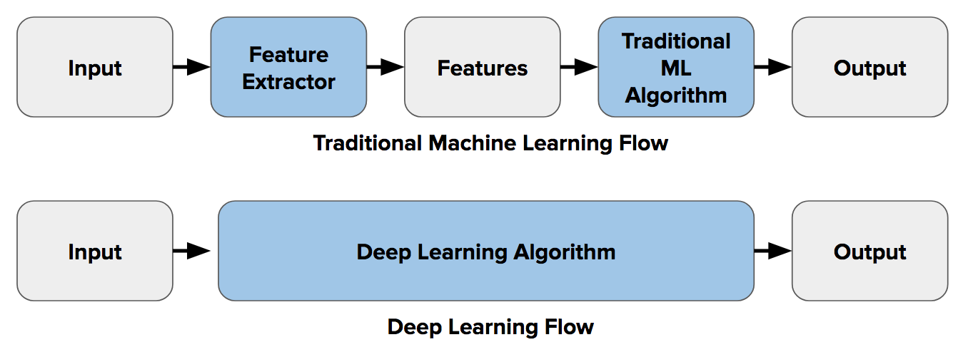
Whereas for the classical ML, domain experts and data scientists often have to write hand-crafted algorithms to extract and represent high-dimensional features from the raw data, deep learning models, on the other hand, automatically extracts and work on these complex features.
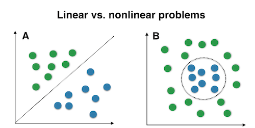
A lot of theory and mathematical machines behind the classical ML (regression, support vector machines, etc.) were developed with linear models in mind. However, practical real-life problems are often nonlinear in nature and therefore cannot be effectively solved using those ML methods.
A simple illustration is shown below and although it is somewhat over-simplified, it conveys the idea. Deep learning models are inherently better to tackle such nonlinear classification tasks.
However, at its core, structurally, a deep learning model consists of stacked layers of linear perceptron units and simple matrix multiplications are performed over them. Matrix operations are essentially linear multiplication and addition.
So, how does a deep learning model introduce nonlinearity in its computation? The answer lies in the so-called ‘activation functions’.
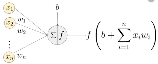
The activation function is the non-linear function that we apply over the output data coming out of a particular layer of neurons before it propagates as the input to the next layer. In the figure below, the function f denotes the activation.
It can also be shown, mathematically, that the universal approximation power of a deep neural network - the ability to approximate any mathematical function to a sufficient degree - does not hold without these nonlinear activation stages in between the layers.
There are various kinds and choices for the activation functions and it has been found, empirically, that some of them works better for large datasets or particular problems than the others. We will discuss these in the next section.

Fundamentally, deep learning models fall in the class of supervised machine learning methods - techniques that extract the hidden pattern from a dataset by observing given examples of known answers.
Evidently, it does so by comparing its predictions to the ground truth (labeled images for example) and turning the parameters of the model. The difference between the prediction and the ground truth is called the ‘classification error’.
Parameters of a DL model consists of a set of weights connecting neurons across layers and bias terms which add to those layers. So, the ultimate goal is to set those weights to specific values which reduces the overall classification error.
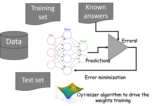
This is a minimization operation, mathematically. Consequently, an optimization technique is needed and it sits at the core of a deep learning algorithm. We also know that the overall representation structure of the DL model is a highly complex nonlinear function and therefore, the optimizer is responsible for minimizing the error produced by the evaluation of this complex function. Therefore, standard optimization like linear programming does not work for DL models and innovative nonlinear optimization must be used.
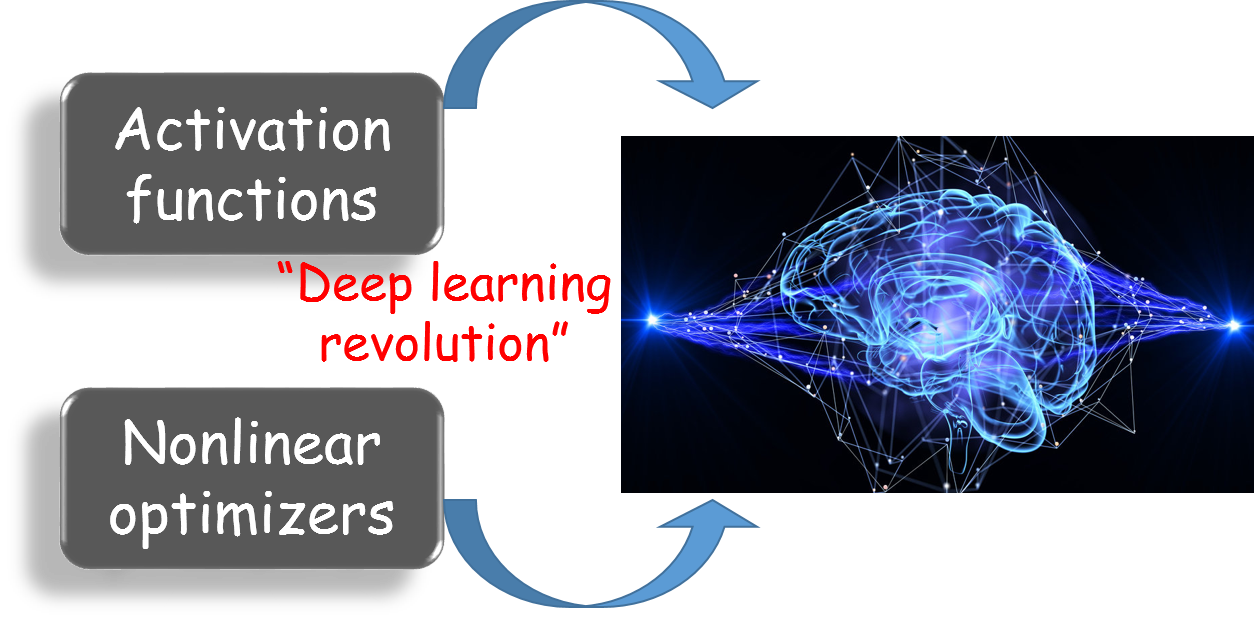
These two components - activation functions and nonlinear optimizers - are at the core of every deep learning architecture. However, there is considerable variation in the specifics of these components, and in the next two sections, we go over the latest developments.
The fundamental inspiration of the activation function as a thresholding gate comes from biological neurons’ behavior.
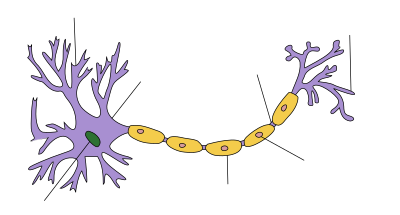
The physical structure of a typical neuron consists of a cell body, an axon for sending messages to other neurons, and dendrites for receiving signals from other neurons.
The weight (strength) associated with a dendrite, called synaptic weights, gets multiplied by the incoming signal and is accumulated in the cell body. If the strength of the resulting signal is above a certain threshold, the neuron passes the message to the axon, else the signal dies off.
In artificial neural networks, we extend this idea by shaping the outputs of neurons with activation functions. They push the output signal strength up or down in a nonlinear fashion depending on the magnitude. High magnitude signals propagate further and take part in shaping the final prediction of the network whereas the weakened signal dies off quickly.
Some common activation functions for deep learning are described below.
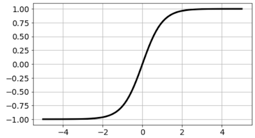
The sigmoid function is one of the nonlinear activation functions for deep learning that takes a real-valued number as an input and compresses all its outputs to the range of [0,1. There are many functions with the characteristic of an “S” shaped curve known as sigmoid functions. The most commonly used function is the logistic function.
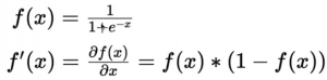
In the logistic function, a small change in the input only causes a small change in the output as opposed to the stepped output. Hence, the output is smoother than the step function output.

While sigmoid functions were one of the first ones used in early neural network research, they have fallen in favor recently. Other functions have been shown to produce the same performance with fewer iterations. However, the idea is still quite useful for the last layer of a DL architecture (either as stand-alone or as a softmax function) for classification tasks. This is because of the output range of [0,1] which can be interpreted as probability values.
Tanh is a non-linear activation function for deep learning that compresses all its inputs to the range [-1, 1]. The mathematical representation is given below,
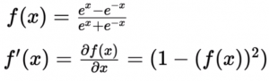
Tanh is similar to the logistic function, it saturates at large positive or large negative values, the gradient still vanishes at saturation. But Tanh function is zero-centered so that the gradients are not restricted to move in certain directions.
ReLU is one of the non-linear activation functions for deep learning which was first popularized in the context of a convolution neural network (CNN). If the input is positive then the function would output the value itself, if the input is negative the output would be zero.
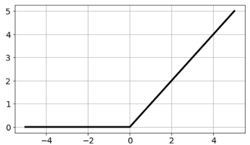
The function doesn’t saturate in the positive region, thereby avoiding the vanishing gradient problem to a large extent. Furthermore, the process of ReLu function evaluation is computationally efficient as it does not involve computing exp(x), and therefore, in practice, it converges much faster than logistic/Tanh for the same performance (classification accuracy for example). For this reason, ReLU has become a de-facto standard for large convolutional neural network architectures such as Inception, ResNet, MobileNet, VGGNet, etc.
However, despite its critical advantages, ReLU sometimes can give rise to dead neuron problems as it zeroes the output for any negative input. This can lead to reduced learning updates for a large portion of a neural network. To avoid facing this issue, we can use the so-called ‘leaky ReLU’ approach.
In this variant of ReLU, instead of producing zero for negative inputs, it will just produce a very small value proportional to the input i.e 0.01x, as if the function is ‘leaking’ some value in the negative region instead of producing hard zero values.
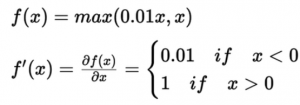
Because of the small value (0.1) proportional to the input for the negative values, the gradient would not saturate. If the input is negative, the gradient would be 0.01 times the input, this ensures neurons don’t die. So, the apparent advantages of Leaky ReLU are that it doesn’t saturate in the positive or negative region, it avoids 'dead neurons' problem, it is easy to compute, and it produces close to zero-centered outputs.
Although you are more likely to come across one of the aforementioned activation functions, in dealing with common DL architectures, it is good to know about some recent developments where researchers have proposed alternative activation functions to speed up large model training and hyperparameter optimization tasks.
Swish is such a function, proposed by the famous Google Brain team (in a paper where they searched for optimum activation function using complex reinforcement learning techniques).
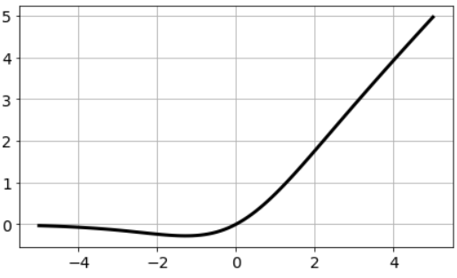
Google's team’s experiments show that Swish tends to work better than ReLU on deeper models across a number of challenging data sets. For example, simply replacing ReLUs with Swish units improves top-1 classification accuracy on ImageNet by 0.9% for Mobile NASNetA and 0.6% for Inception-ResNet-v2. The simplicity of Swish and its similarity to ReLU makes it easy for practitioners to replace ReLUs with Swish units in any neural network.
As stated earlier, a deep learning model works by gradually reducing the prediction error with respect to a training dataset by adjusting the weights of the connections.
But how does it do this automatically? The answer lies in the technique called - backpropagation with gradient descent.
The idea is to construct a cost function (or loss function) which measures the difference between the actual output and predicted output from the model. Then gradients of this cost function, with respect to the model weights, are computed and propagated back layer by layer. This way, the model knows the weights, responsible for creating a larger error, and tunes them accordingly.
The cost function of a deep learning model is a complex high-dimensional nonlinear function that can be thought of as uneven terrain with ups and downs. Somehow, we want to reach the bottom of the valley i.e. minimize the cost. Gradient indicates the direction of increase. As we want to find the minimum point in the valley we need to go in the opposite direction of the gradient. We update parameters in the negative gradient direction to minimize the loss.
But how much to update at each step? That depends on the learning rate.
The learning rate controls how much we should adjust the weights with respect to the loss gradient. Learning rates are randomly initialized. The lower the value of the learning rate the slower will be the convergence to global minima. A higher value for the learning rate will not allow the gradient descent to converge.
Basically, the update equation for weight optimization is,
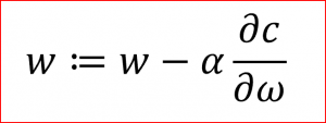
Here, α is the learning rate, C is the cost function and w and ω are the weight vectors. We update the weights proportional to the negative of the gradient (scaled by the learning rate).
There are a few variations of the core gradient descent algorithm,
In batch gradient, we use the entire dataset to compute the gradient of the cost function for each iteration of the gradient descent and then update the weights. Since we use the entire dataset to compute the gradient at one shot, the convergence is slow. If the dataset is huge and contains millions or billions of data points then it is memory as well as computationally intensive as it involves the matrix (with billions of rows and columns) inversion and multiplication steps.
Stochastic gradient descent uses a single data point (randomly chosen) to calculate the gradient and update the weights with every iteration. The dataset is shuffled to make it randomized. As the dataset is randomized and weights are updated for every single example, the cost function and weight update are generally noisy.
Mini-batch gradient is a variation of stochastic gradient descent where instead of a single training example, a mini-batch of samples is used. Mini batch gradient descent is widely used and converges faster and is more stable. The batch size can vary depending on the dataset and generally are 128 or 256. The data per batch easily fits in the memory, the process is computationally efficient, and it benefits from vectorization. If the search (for minima) is stuck in a local minimum point, some noisy random steps can take them out of it.
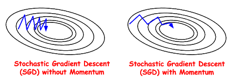
The idea is momentum is borrowed from simple physics, where it can be thought of as a property of matter which maintains the inertial state of an object rolling downhill. Under gravity, the object gains momentum (increases speed) as it rolls further down.
For gradient descent, Momentum helps accelerate the process when it finds surfaces that curve more steeply in one direction than in another direction and dampens the speed suitably. This prevents overshooting a good minima while trying to gradually improve the speed of convergence.
It accomplishes this by keeping track of a history of gradients along the way and using past gradients to determine the shape of the movement of the current search.
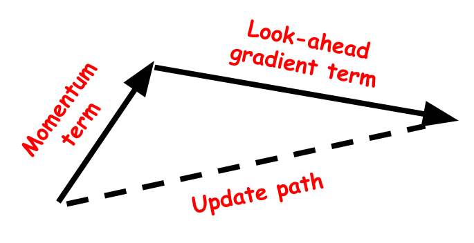
This is an enhanced Momentum-based technique where the future gradients are computed ahead of the time (based on some look-ahead logic) and that information is used to help speed up the convergence as well as slowing down the update rate as necessary.
Here is a detailed article on various sub-types and formulations of NAG.
Many a times, the dataset exhibits sparsity and some parameters need to be updated more frequently than others. This can be done by tuning the learning rate differently for different sets of parameters and AdaGrad does precisely that.
AdaGrad perform larger updates for infrequent parameters and smaller updates for frequent parameters. It is well suited when we have sparse data as in large scale neural networks. For example, GloVe word embedding (an essential encoding scheme for Natural Language Processing or NLP tasks) uses AdaGrad where infrequent words required a greater update and frequent words require smaller updates.
Below we show the update equation for AdaGrad where in the denominator, all the past gradients are accumulated (sum of squares term).
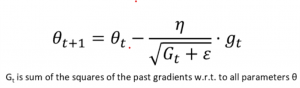
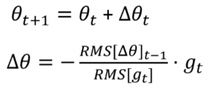
The denominator term in the AdaGrad keeps on accumulating the previous gradients and therefore can make the effective learning rate close to zero after some time. This will make the learning ineffective for the neural network. AdaDelta tries to address this monotonically decreasing tuning of learning rate by restricting the accumulation of past gradients within some fixed window by calculating a running average.
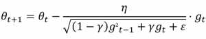
RMSProp tries to address the issue of Adagrad’s rapidly diminishing learning rate by using a moving average of the squared gradients. It utilizes the magnitude of the recent gradient descents to normalize the gradient. Effectively, this algorithm divides the learning rate by the average of the exponential decay of squared gradients.
In this article, we went over two core components of a deep learning model - activation function and optimizer algorithm. The power of a deep learning to learn highly complex pattern from huge datasets stems largely from these components as they help the model learn nonlinear features in a fast and efficient manner.
Both of these are areas of active research and new developments are happening to enable training of ever larger models and faster but stable optimization process while learning over multiple epochs using terabytes of data sets.

Deep Learning (DL) models are revolutionizing the business and technology world with jaw-dropping performances in one application area after another — image classification, object detection, object tracking, pose recognition, video analytics, synthetic picture generation — just to name a few. You may have heard about Activation functions or optimizer for deep learning, and this blog will explore this topic
DL models use millions of parameters and create extremely complex and highly nonlinear internal representations of the images or datasets that are fed to these models.
Whereas for the classical ML, domain experts and data scientists often have to write hand-crafted algorithms to extract and represent high-dimensional features from the raw data, deep learning models, on the other hand, automatically extracts and work on these complex features.
A lot of theory and mathematical machines behind the classical ML (regression, support vector machines, etc.) were developed with linear models in mind. However, practical real-life problems are often nonlinear in nature and therefore cannot be effectively solved using those ML methods.
A simple illustration is shown below and although it is somewhat over-simplified, it conveys the idea. Deep learning models are inherently better to tackle such nonlinear classification tasks.
However, at its core, structurally, a deep learning model consists of stacked layers of linear perceptron units and simple matrix multiplications are performed over them. Matrix operations are essentially linear multiplication and addition.
So, how does a deep learning model introduce nonlinearity in its computation? The answer lies in the so-called ‘activation functions’.
The activation function is the non-linear function that we apply over the output data coming out of a particular layer of neurons before it propagates as the input to the next layer. In the figure below, the function f denotes the activation.
It can also be shown, mathematically, that the universal approximation power of a deep neural network - the ability to approximate any mathematical function to a sufficient degree - does not hold without these nonlinear activation stages in between the layers.
There are various kinds and choices for the activation functions and it has been found, empirically, that some of them works better for large datasets or particular problems than the others. We will discuss these in the next section.
Fundamentally, deep learning models fall in the class of supervised machine learning methods - techniques that extract the hidden pattern from a dataset by observing given examples of known answers.
Evidently, it does so by comparing its predictions to the ground truth (labeled images for example) and turning the parameters of the model. The difference between the prediction and the ground truth is called the ‘classification error’.
Parameters of a DL model consists of a set of weights connecting neurons across layers and bias terms which add to those layers. So, the ultimate goal is to set those weights to specific values which reduces the overall classification error.
This is a minimization operation, mathematically. Consequently, an optimization technique is needed and it sits at the core of a deep learning algorithm. We also know that the overall representation structure of the DL model is a highly complex nonlinear function and therefore, the optimizer is responsible for minimizing the error produced by the evaluation of this complex function. Therefore, standard optimization like linear programming does not work for DL models and innovative nonlinear optimization must be used.
These two components - activation functions and nonlinear optimizers - are at the core of every deep learning architecture. However, there is considerable variation in the specifics of these components, and in the next two sections, we go over the latest developments.
The fundamental inspiration of the activation function as a thresholding gate comes from biological neurons’ behavior.
The physical structure of a typical neuron consists of a cell body, an axon for sending messages to other neurons, and dendrites for receiving signals from other neurons.
The weight (strength) associated with a dendrite, called synaptic weights, gets multiplied by the incoming signal and is accumulated in the cell body. If the strength of the resulting signal is above a certain threshold, the neuron passes the message to the axon, else the signal dies off.
In artificial neural networks, we extend this idea by shaping the outputs of neurons with activation functions. They push the output signal strength up or down in a nonlinear fashion depending on the magnitude. High magnitude signals propagate further and take part in shaping the final prediction of the network whereas the weakened signal dies off quickly.
Some common activation functions for deep learning are described below.
The sigmoid function is one of the nonlinear activation functions for deep learning that takes a real-valued number as an input and compresses all its outputs to the range of [0,1. There are many functions with the characteristic of an “S” shaped curve known as sigmoid functions. The most commonly used function is the logistic function.
In the logistic function, a small change in the input only causes a small change in the output as opposed to the stepped output. Hence, the output is smoother than the step function output.
While sigmoid functions were one of the first ones used in early neural network research, they have fallen in favor recently. Other functions have been shown to produce the same performance with fewer iterations. However, the idea is still quite useful for the last layer of a DL architecture (either as stand-alone or as a softmax function) for classification tasks. This is because of the output range of [0,1] which can be interpreted as probability values.
Tanh is a non-linear activation function for deep learning that compresses all its inputs to the range [-1, 1]. The mathematical representation is given below,
Tanh is similar to the logistic function, it saturates at large positive or large negative values, the gradient still vanishes at saturation. But Tanh function is zero-centered so that the gradients are not restricted to move in certain directions.
ReLU is one of the non-linear activation functions for deep learning which was first popularized in the context of a convolution neural network (CNN). If the input is positive then the function would output the value itself, if the input is negative the output would be zero.
The function doesn’t saturate in the positive region, thereby avoiding the vanishing gradient problem to a large extent. Furthermore, the process of ReLu function evaluation is computationally efficient as it does not involve computing exp(x), and therefore, in practice, it converges much faster than logistic/Tanh for the same performance (classification accuracy for example). For this reason, ReLU has become a de-facto standard for large convolutional neural network architectures such as Inception, ResNet, MobileNet, VGGNet, etc.
However, despite its critical advantages, ReLU sometimes can give rise to dead neuron problems as it zeroes the output for any negative input. This can lead to reduced learning updates for a large portion of a neural network. To avoid facing this issue, we can use the so-called ‘leaky ReLU’ approach.
In this variant of ReLU, instead of producing zero for negative inputs, it will just produce a very small value proportional to the input i.e 0.01x, as if the function is ‘leaking’ some value in the negative region instead of producing hard zero values.
Because of the small value (0.1) proportional to the input for the negative values, the gradient would not saturate. If the input is negative, the gradient would be 0.01 times the input, this ensures neurons don’t die. So, the apparent advantages of Leaky ReLU are that it doesn’t saturate in the positive or negative region, it avoids 'dead neurons' problem, it is easy to compute, and it produces close to zero-centered outputs.
Although you are more likely to come across one of the aforementioned activation functions, in dealing with common DL architectures, it is good to know about some recent developments where researchers have proposed alternative activation functions to speed up large model training and hyperparameter optimization tasks.
Swish is such a function, proposed by the famous Google Brain team (in a paper where they searched for optimum activation function using complex reinforcement learning techniques).
Google's team’s experiments show that Swish tends to work better than ReLU on deeper models across a number of challenging data sets. For example, simply replacing ReLUs with Swish units improves top-1 classification accuracy on ImageNet by 0.9% for Mobile NASNetA and 0.6% for Inception-ResNet-v2. The simplicity of Swish and its similarity to ReLU makes it easy for practitioners to replace ReLUs with Swish units in any neural network.
As stated earlier, a deep learning model works by gradually reducing the prediction error with respect to a training dataset by adjusting the weights of the connections.
But how does it do this automatically? The answer lies in the technique called - backpropagation with gradient descent.
The idea is to construct a cost function (or loss function) which measures the difference between the actual output and predicted output from the model. Then gradients of this cost function, with respect to the model weights, are computed and propagated back layer by layer. This way, the model knows the weights, responsible for creating a larger error, and tunes them accordingly.
The cost function of a deep learning model is a complex high-dimensional nonlinear function that can be thought of as uneven terrain with ups and downs. Somehow, we want to reach the bottom of the valley i.e. minimize the cost. Gradient indicates the direction of increase. As we want to find the minimum point in the valley we need to go in the opposite direction of the gradient. We update parameters in the negative gradient direction to minimize the loss.
But how much to update at each step? That depends on the learning rate.
The learning rate controls how much we should adjust the weights with respect to the loss gradient. Learning rates are randomly initialized. The lower the value of the learning rate the slower will be the convergence to global minima. A higher value for the learning rate will not allow the gradient descent to converge.
Basically, the update equation for weight optimization is,
Here, α is the learning rate, C is the cost function and w and ω are the weight vectors. We update the weights proportional to the negative of the gradient (scaled by the learning rate).
There are a few variations of the core gradient descent algorithm,
In batch gradient, we use the entire dataset to compute the gradient of the cost function for each iteration of the gradient descent and then update the weights. Since we use the entire dataset to compute the gradient at one shot, the convergence is slow. If the dataset is huge and contains millions or billions of data points then it is memory as well as computationally intensive as it involves the matrix (with billions of rows and columns) inversion and multiplication steps.
Stochastic gradient descent uses a single data point (randomly chosen) to calculate the gradient and update the weights with every iteration. The dataset is shuffled to make it randomized. As the dataset is randomized and weights are updated for every single example, the cost function and weight update are generally noisy.
Mini-batch gradient is a variation of stochastic gradient descent where instead of a single training example, a mini-batch of samples is used. Mini batch gradient descent is widely used and converges faster and is more stable. The batch size can vary depending on the dataset and generally are 128 or 256. The data per batch easily fits in the memory, the process is computationally efficient, and it benefits from vectorization. If the search (for minima) is stuck in a local minimum point, some noisy random steps can take them out of it.
The idea is momentum is borrowed from simple physics, where it can be thought of as a property of matter which maintains the inertial state of an object rolling downhill. Under gravity, the object gains momentum (increases speed) as it rolls further down.
For gradient descent, Momentum helps accelerate the process when it finds surfaces that curve more steeply in one direction than in another direction and dampens the speed suitably. This prevents overshooting a good minima while trying to gradually improve the speed of convergence.
It accomplishes this by keeping track of a history of gradients along the way and using past gradients to determine the shape of the movement of the current search.
This is an enhanced Momentum-based technique where the future gradients are computed ahead of the time (based on some look-ahead logic) and that information is used to help speed up the convergence as well as slowing down the update rate as necessary.
Here is a detailed article on various sub-types and formulations of NAG.
Many a times, the dataset exhibits sparsity and some parameters need to be updated more frequently than others. This can be done by tuning the learning rate differently for different sets of parameters and AdaGrad does precisely that.
AdaGrad perform larger updates for infrequent parameters and smaller updates for frequent parameters. It is well suited when we have sparse data as in large scale neural networks. For example, GloVe word embedding (an essential encoding scheme for Natural Language Processing or NLP tasks) uses AdaGrad where infrequent words required a greater update and frequent words require smaller updates.
Below we show the update equation for AdaGrad where in the denominator, all the past gradients are accumulated (sum of squares term).
The denominator term in the AdaGrad keeps on accumulating the previous gradients and therefore can make the effective learning rate close to zero after some time. This will make the learning ineffective for the neural network. AdaDelta tries to address this monotonically decreasing tuning of learning rate by restricting the accumulation of past gradients within some fixed window by calculating a running average.
RMSProp tries to address the issue of Adagrad’s rapidly diminishing learning rate by using a moving average of the squared gradients. It utilizes the magnitude of the recent gradient descents to normalize the gradient. Effectively, this algorithm divides the learning rate by the average of the exponential decay of squared gradients.
In this article, we went over two core components of a deep learning model - activation function and optimizer algorithm. The power of a deep learning to learn highly complex pattern from huge datasets stems largely from these components as they help the model learn nonlinear features in a fast and efficient manner.
Both of these are areas of active research and new developments are happening to enable training of ever larger models and faster but stable optimization process while learning over multiple epochs using terabytes of data sets.