Graph Neural Networks Explained
Graph neural networks (GNNs) belong to a category of neural networks that operate naturally on data structured as graphs. Despite being what can be a confusing topic, GNNs can be distilled into just a handful of simple concepts.
Starting With Recurrent Neural Networks (RNNs)
We’ll pick a likely familiar starting point: recurrent neural networks. As you may recall, recurrent neural networks are well-suited to data that are arranged in a sequence, such as time series data or language. The defining feature for a recurrent neural network is that the state of an RNN depends not only on the current inputs but also on the network’s previous hidden state. There have been many improvements to RNNs over the years, generally falling under the category of LSTM-style RNNs with a multiplicative gating function between the current and previous hidden state of the model. A review of LSTM variants and their relation to vanilla RNNs can be found here.
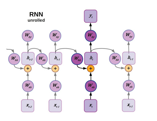
Unrolled RNN.
Although recurrent neural networks have been somewhat superseded by large transformer models for natural language processing, they still find widespread utility in a variety of areas that require sequential decision making and memory (reinforcement learning comes to mind). Now imagine the sequence that an RNN operates on as a directed linear graph, but remove the inputs and weighted connections, which will be embedded as node states and edges, respectively. In fact, remove the output as well. In a graph neural network the input data is the original state of each node, and the output is parsed from the hidden state after performing a certain number of updates defined as a hyperparameter.
Interested in a deep learning workstation?
Learn more about Exxact AI workstations starting at $3,700
Reimagining Recurrent Neural Network (RNN) as a Graph Neural Neural Network (GNN)
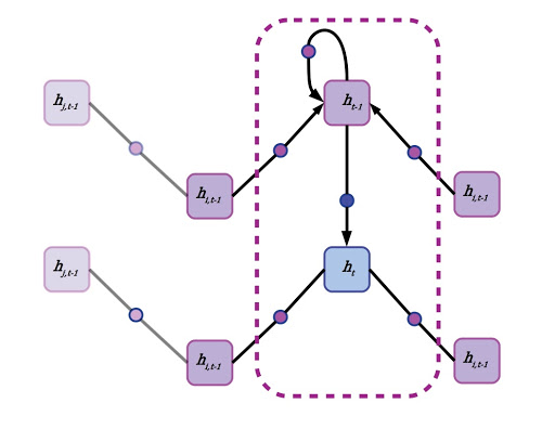
Re-imagining an RNN as a graph neural network on a linear acyclic graph.
First, each node aggregates the states of its neighbors. This can be accomplished by forward passes through a neural network with weights shared across edges, or by simply averaging the state vectors of all adjacent nodes. A node’s own previous hidden state is also included in this neighborhood aggregation, but often gets special treatment. A node’s self-state may be parsed through its own hidden layer or by simply appending it to the state vector aggregated from the mean of all neighboring states. There’s no concept of time in a generalized GNN, and each node pulls data from its neighbors regardless of whether they are “in front” or “behind,” although in a directed graph or graph with multiple species of connections, different edges may have their own aggregation policies. Another term for neighborhood aggregation is neural message passing.
It’s easy to get bogged down in the details, and there’s quite a bit of room for versatility in GNNs.
In general, GNN updates can be broken into two simple steps:
- Aggregate or parse states of neighboring nodes, aka “message passing.”
- Update node state
Now that we’ve made the connection that an RNN can be formulated as a special case of a graph neural network, let’s back up for a moment and make sure we’re all familiar with the same terms. Graphs are a mathematical abstraction for representing and analyzing networks of nodes (aka vertices) connected by relationships known as edges. Graphs come with their own rich branch of mathematics called graph theory, for manipulation and analysis. A simple graph with 4 nodes is shown below.
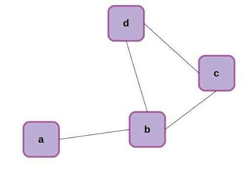
Simple 4-node graph.
The nodes of the above graph can be readily described as a list: [0,1,2,3], while the edges can be described as an adjacency matrix, where each edge is represented by a 1 and missing connections between nodes are left as 0.
| Node | a | b | c | d |
| a | 0 | 1 | 0 | 0 |
| b | 1 | 0 | 1 | 1 |
| c | 0 | 1 | 0 | 1 |
| d | 0 | 1 | 1 | 0 |
Non-Directed Nature of GNNs
The adjacency matrix above reflects the non-directed nature of the corresponding graph. A connection between node 0 and node 1 is the same type of connection as that between 1 and 0, and this is reflected in a symmetry about the matrix diagonal. It’s also not unusual to reflect node self-connections in the adjacency matrix, and we can easily update the matrix to show this by adding the identity matrix of equivalent size, giving the adjacency matrix a value of 1 at every diagonal element.
Just to build a final bit of intuition, let’s visualize how information propagates through the graph. In this case there is no step 2 for updating node states (or we can think of the update step as being an identity function), and node states are represented by scalars.
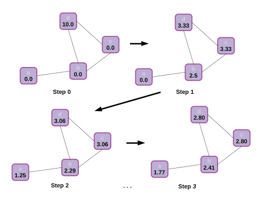
State propagation or message passing in a graph, with an identity function update following each neighborhood aggregation step. The graph starts with all nodes in a scalar state of 0.0, excepting d which has state 10.0. Through neighborhood aggregation the other nodes gradually are influenced by the initial state of d, depending on each node’s location in the graph. Eventually the graph will reach equilibrium and each node will approach a scalar state value 2.5.
That simple example of scalar state propagation in a graph gives us an intuitive feel for how the structure of a graph affects information flow, and how this might affect the final output of the model. It makes sense that nearby nodes will have a greater effect on one another than distant ones, and influence will be impeded by traveling through sparse connections.
What Does This Mean for the Adjacency Matrix?
Returning to the adjacency matrix mentioned earlier: that’s actually an especially easy way to aggregate the states of neighboring nodes. We can simply matrix-multiply the array of node states by the adjacency matrix to sum the value of all neighbors, or first divide each column in the matrix by the sum of that column to get the mean of neighboring node states. That’s an easy and computationally fast way to define and implement neighborhood node aggregation.
Another strategy is to define each type of edge as a feed forward neural network, sharing weights with all the instances of that type of edge. The feed forward network is applied to each neighbor node state vector before averaging, or, in a graph attention network, applying attention and then summing. Finally, in a real GNN, after aggregating state data from a node’s self and neighbors, the node’s state is updated. The update rule can be any type of neural network, but it’s common to use a recurrent model like a gated recurrent unit (GRU).
Applying Graph Neural Networks to Useful Inference
Let’s take a realistic (but still simplified) scenario amenable to applying graph neural networks, to see how this structural information contributes to useful inference. Say we wanted to predict which atoms in amino acid residues were hydrophilic (miscible in water) as opposed to those that are hydrophobic, like oils. That’s important information for determining how proteins fold, a difficult and fundamental question in molecular biology. We’ll examine arginine as an example, an amino acid with both hydrophilic and hydrophobic traits. After formulating the molecule as a graph:
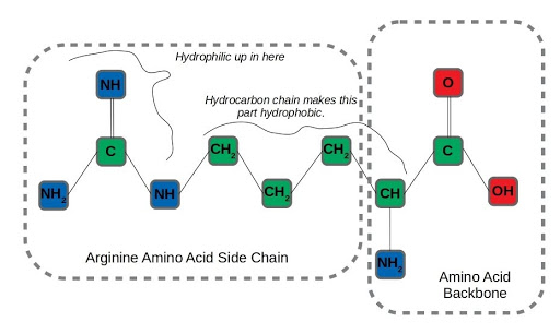
Graph representation of arginine, an amphipathic amino acid.
We can run neighborhood aggregation and state updates to get a prediction of hydrophilicity at each node. At physiological pH, the amino groups in the backbone and amino acid sidechain of arginine are protonated. On the other hand, the long hydrocarbon chain connecting the backbone to the end of the side-chain is very hydrophobic, so arginine has both water-loving and water-repelling characteristics.
An interesting aspect of the arginine side-chain that affects this dual nature is that the hydrophilicity is distributed across all three nitrogen-containing amino residues in the side-chain. The term for this arrangement of 3 nitrogens around a central carbon is a guanidino group. It’s hard to imagine capturing this distributed hydrophilicity by considering each node in isolation, but it’s exactly the type of insight that can be learned by incorporating the structural information of a graph.
A Tour of Graph Neural Network Applications
Although graph neural networks were described in 2005, and related concepts were kicking around before that, GNNs have started to really come into their own lately. In the last few years, GNNs have found enthusiastic adoption in social network analysis and computational chemistry, especially for drug discovery. As such it’s not a bad time to get familiar with the promising style of model in case you may run into those types of problems that can be readily formulated on graphs.
One of the earliest applications of GNNs was page ranking for web search, but they’ve come a long way since then. Natural language processing and parsing sentence structure, another early application, achieved state of the art results on a text summarization benchmark in 2010. GNNs have since been used for everything from making traffic predictions to quantum chemistry.
Materials science has recently been an attractive area for applying GNNs. Deepmind published results earlier this year using GNNs to shed light on the glass transition, a subject of substantial contention in physics. That’s part of a larger trend using GNNs to study material properties. A related application domain, and perhaps the most exciting in terms of potential impact, is graph neural networks for chemistry. GNNs are particularly well suited for neural reasoning about molecules, including the small molecules that make good drug candidates. If you are interested in working in or gaining a better understanding of machine learning for drug discovery working with GNNs is practically a must-have skill.
What’s Next for Graph Neural Networks (GNNs)?
Attention is a concept that gives machine learning models the ability to learn how to apportion different weights to different inputs, in other words giving models the capability to manage their own attention. We can point to Vaswani et al.’s “Attention is All You Need” as an example of recent seminal work in this area. The paper posited the attention-only transformer as a do-it-all language model (see here for more about attention and transformers). This has for the most part held true with the development of massive transformer models like BERT and GPT-3 dominating natural language metrics in recent years.
Adding attention to the existing GNN algorithm we discussed earlier is fairly simple. During neighborhood aggregation, in addition to transforming the states of neighboring nodes via a feed-forward network on graph edges, an attention mechanism is included to calculate vector weighting coefficients. Several attention mechanisms are available, such as the dot-product attention mechanism used in the original transformer models, as well-illustrated by Jay Allamar. In this scheme, fully-connected layers produce a key and query vector, in addition to a value vector for each input, which in this case are connected to nodes by graph edges. Taking the dot product of the key and query vectors yields a scalar constant, which is then subjected to a softmax activation function alongside all other key-query dot products in the graph neighborhood, aka the raw attention coefficients. Finally, instead of summing all the value vectors directly, they are first weighted by the attention coefficients.
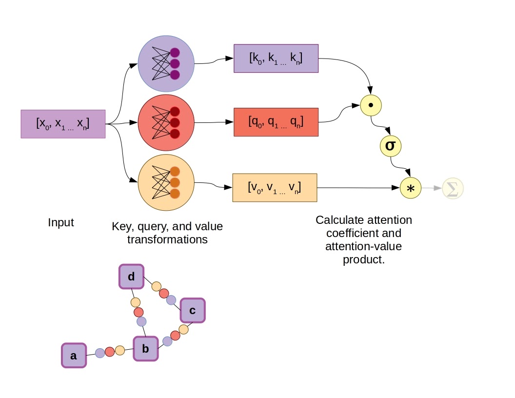
Example of a Graph Attention Network using the dot-product attention mechanism. In this case σ represents the softmax function.
Quantum Graph Neural Networks (QGNNs)
If quantum chemistry on graph neural networks is an effective way to take advantage of molecular structure when making inferences about quantum chemistry, defining the neural networks of a GNN as an ansatz, or quantum circuit architecture, can bring models even closer to the system they are making predictions and learning about. Quantum graph neural networks (QGNNs) were introduced in 2019 by Verdon et al. The authors further subdivided their work into two different classes: quantum graph recurrent neural networks and quantum graph convolutional networks.
The specific type of quantum circuit used by QGNNs falls under the category of “variational quantum algorithms.” In short, these are quantum circuits with parameters that can be trained by gradient descent, and these trainable parameters are the quantum equivalent of weights and biases. A known issue in training variational quantum algorithms/circuits is the presence of “barren plateaus,” regions in the fitness landscape where the objective score doesn’t change very much. QGNNs were devised as a means of imparting structural information to variational quantum circuits to ameliorate the presence of barren plateaus. Verdon and colleagues demonstrated QGNNs applied to learning quantum dynamics, graph clustering, and graph isomorphism classification.
Replace Neural Networks with Graph Neural Networks (GNNs)?
Should you convert your datasets to graphs, and replace all of your neural networks with GNNs? The answer, of course, depends on your problem’s natural suitability as a graph. Forcing a dataset that is better represented on a linear sequence or 2D grid to fit on a graph will probably only lead to more difficult implementation and slower training. GNNs do look like they’ll be the dominant model type for machine learning on molecules for the next few years, so if you’re going to be working in computational chemistry it’s an important tool to be familiar with. That goes double for drug discovery and development.
GNNs also seem to be a good match for social media graphs and other types of relational networks naturally representable as graphs. Although GNNs have been used for image and language-based tasks, transformers and the old reliable conv-nets seem to have those areas pretty well covered for now. As a final note, GNNs also might make a compelling framework for combining deep learning neural networks with “Good Old-Fashioned AI” (GOFAI), a topic that was reviewed in a JCAI survey paper on neurosymbolic AI. This hybrid approach may offer some advantages in terms of interpretability and control, at some cost in overall flexibility.
Bringing GNNs Into the Future
If you’ve heard of graph neural networks but have been put off by their seeming complexity, hopefully this article has helped to overcome that initial hurdle. Remember, GNNs are just deep learning models that reside on and operate on graphs. There’s plenty of flexibility in how you build one, but they all share the basic steps of neighborhood aggregation followed by state updates. If you’ve been waiting to see a noteworthy commercial success before diving in, look no further than the impact of GNNs on computational chemistry and drug discovery over the next few years. It’s a worthwhile model class to be familiar with, and set to find increasing traction and impact over the course of this decade.
Have any questions?
Contact Exxact Today

A Friendly Introduction to Graph Neural Networks
Graph Neural Networks Explained
Graph neural networks (GNNs) belong to a category of neural networks that operate naturally on data structured as graphs. Despite being what can be a confusing topic, GNNs can be distilled into just a handful of simple concepts.
Starting With Recurrent Neural Networks (RNNs)
We’ll pick a likely familiar starting point: recurrent neural networks. As you may recall, recurrent neural networks are well-suited to data that are arranged in a sequence, such as time series data or language. The defining feature for a recurrent neural network is that the state of an RNN depends not only on the current inputs but also on the network’s previous hidden state. There have been many improvements to RNNs over the years, generally falling under the category of LSTM-style RNNs with a multiplicative gating function between the current and previous hidden state of the model. A review of LSTM variants and their relation to vanilla RNNs can be found here.

Unrolled RNN.
Although recurrent neural networks have been somewhat superseded by large transformer models for natural language processing, they still find widespread utility in a variety of areas that require sequential decision making and memory (reinforcement learning comes to mind). Now imagine the sequence that an RNN operates on as a directed linear graph, but remove the inputs and weighted connections, which will be embedded as node states and edges, respectively. In fact, remove the output as well. In a graph neural network the input data is the original state of each node, and the output is parsed from the hidden state after performing a certain number of updates defined as a hyperparameter.
Interested in a deep learning workstation?
Learn more about Exxact AI workstations starting at $3,700
Reimagining Recurrent Neural Network (RNN) as a Graph Neural Neural Network (GNN)

Re-imagining an RNN as a graph neural network on a linear acyclic graph.
First, each node aggregates the states of its neighbors. This can be accomplished by forward passes through a neural network with weights shared across edges, or by simply averaging the state vectors of all adjacent nodes. A node’s own previous hidden state is also included in this neighborhood aggregation, but often gets special treatment. A node’s self-state may be parsed through its own hidden layer or by simply appending it to the state vector aggregated from the mean of all neighboring states. There’s no concept of time in a generalized GNN, and each node pulls data from its neighbors regardless of whether they are “in front” or “behind,” although in a directed graph or graph with multiple species of connections, different edges may have their own aggregation policies. Another term for neighborhood aggregation is neural message passing.
It’s easy to get bogged down in the details, and there’s quite a bit of room for versatility in GNNs.
In general, GNN updates can be broken into two simple steps:
- Aggregate or parse states of neighboring nodes, aka “message passing.”
- Update node state
Now that we’ve made the connection that an RNN can be formulated as a special case of a graph neural network, let’s back up for a moment and make sure we’re all familiar with the same terms. Graphs are a mathematical abstraction for representing and analyzing networks of nodes (aka vertices) connected by relationships known as edges. Graphs come with their own rich branch of mathematics called graph theory, for manipulation and analysis. A simple graph with 4 nodes is shown below.

Simple 4-node graph.
The nodes of the above graph can be readily described as a list: [0,1,2,3], while the edges can be described as an adjacency matrix, where each edge is represented by a 1 and missing connections between nodes are left as 0.
| Node | a | b | c | d |
| a | 0 | 1 | 0 | 0 |
| b | 1 | 0 | 1 | 1 |
| c | 0 | 1 | 0 | 1 |
| d | 0 | 1 | 1 | 0 |
Non-Directed Nature of GNNs
The adjacency matrix above reflects the non-directed nature of the corresponding graph. A connection between node 0 and node 1 is the same type of connection as that between 1 and 0, and this is reflected in a symmetry about the matrix diagonal. It’s also not unusual to reflect node self-connections in the adjacency matrix, and we can easily update the matrix to show this by adding the identity matrix of equivalent size, giving the adjacency matrix a value of 1 at every diagonal element.
Just to build a final bit of intuition, let’s visualize how information propagates through the graph. In this case there is no step 2 for updating node states (or we can think of the update step as being an identity function), and node states are represented by scalars.

State propagation or message passing in a graph, with an identity function update following each neighborhood aggregation step. The graph starts with all nodes in a scalar state of 0.0, excepting d which has state 10.0. Through neighborhood aggregation the other nodes gradually are influenced by the initial state of d, depending on each node’s location in the graph. Eventually the graph will reach equilibrium and each node will approach a scalar state value 2.5.
That simple example of scalar state propagation in a graph gives us an intuitive feel for how the structure of a graph affects information flow, and how this might affect the final output of the model. It makes sense that nearby nodes will have a greater effect on one another than distant ones, and influence will be impeded by traveling through sparse connections.
What Does This Mean for the Adjacency Matrix?
Returning to the adjacency matrix mentioned earlier: that’s actually an especially easy way to aggregate the states of neighboring nodes. We can simply matrix-multiply the array of node states by the adjacency matrix to sum the value of all neighbors, or first divide each column in the matrix by the sum of that column to get the mean of neighboring node states. That’s an easy and computationally fast way to define and implement neighborhood node aggregation.
Another strategy is to define each type of edge as a feed forward neural network, sharing weights with all the instances of that type of edge. The feed forward network is applied to each neighbor node state vector before averaging, or, in a graph attention network, applying attention and then summing. Finally, in a real GNN, after aggregating state data from a node’s self and neighbors, the node’s state is updated. The update rule can be any type of neural network, but it’s common to use a recurrent model like a gated recurrent unit (GRU).
Applying Graph Neural Networks to Useful Inference
Let’s take a realistic (but still simplified) scenario amenable to applying graph neural networks, to see how this structural information contributes to useful inference. Say we wanted to predict which atoms in amino acid residues were hydrophilic (miscible in water) as opposed to those that are hydrophobic, like oils. That’s important information for determining how proteins fold, a difficult and fundamental question in molecular biology. We’ll examine arginine as an example, an amino acid with both hydrophilic and hydrophobic traits. After formulating the molecule as a graph:

Graph representation of arginine, an amphipathic amino acid.
We can run neighborhood aggregation and state updates to get a prediction of hydrophilicity at each node. At physiological pH, the amino groups in the backbone and amino acid sidechain of arginine are protonated. On the other hand, the long hydrocarbon chain connecting the backbone to the end of the side-chain is very hydrophobic, so arginine has both water-loving and water-repelling characteristics.
An interesting aspect of the arginine side-chain that affects this dual nature is that the hydrophilicity is distributed across all three nitrogen-containing amino residues in the side-chain. The term for this arrangement of 3 nitrogens around a central carbon is a guanidino group. It’s hard to imagine capturing this distributed hydrophilicity by considering each node in isolation, but it’s exactly the type of insight that can be learned by incorporating the structural information of a graph.
A Tour of Graph Neural Network Applications
Although graph neural networks were described in 2005, and related concepts were kicking around before that, GNNs have started to really come into their own lately. In the last few years, GNNs have found enthusiastic adoption in social network analysis and computational chemistry, especially for drug discovery. As such it’s not a bad time to get familiar with the promising style of model in case you may run into those types of problems that can be readily formulated on graphs.
One of the earliest applications of GNNs was page ranking for web search, but they’ve come a long way since then. Natural language processing and parsing sentence structure, another early application, achieved state of the art results on a text summarization benchmark in 2010. GNNs have since been used for everything from making traffic predictions to quantum chemistry.
Materials science has recently been an attractive area for applying GNNs. Deepmind published results earlier this year using GNNs to shed light on the glass transition, a subject of substantial contention in physics. That’s part of a larger trend using GNNs to study material properties. A related application domain, and perhaps the most exciting in terms of potential impact, is graph neural networks for chemistry. GNNs are particularly well suited for neural reasoning about molecules, including the small molecules that make good drug candidates. If you are interested in working in or gaining a better understanding of machine learning for drug discovery working with GNNs is practically a must-have skill.
What’s Next for Graph Neural Networks (GNNs)?
Attention is a concept that gives machine learning models the ability to learn how to apportion different weights to different inputs, in other words giving models the capability to manage their own attention. We can point to Vaswani et al.’s “Attention is All You Need” as an example of recent seminal work in this area. The paper posited the attention-only transformer as a do-it-all language model (see here for more about attention and transformers). This has for the most part held true with the development of massive transformer models like BERT and GPT-3 dominating natural language metrics in recent years.
Adding attention to the existing GNN algorithm we discussed earlier is fairly simple. During neighborhood aggregation, in addition to transforming the states of neighboring nodes via a feed-forward network on graph edges, an attention mechanism is included to calculate vector weighting coefficients. Several attention mechanisms are available, such as the dot-product attention mechanism used in the original transformer models, as well-illustrated by Jay Allamar. In this scheme, fully-connected layers produce a key and query vector, in addition to a value vector for each input, which in this case are connected to nodes by graph edges. Taking the dot product of the key and query vectors yields a scalar constant, which is then subjected to a softmax activation function alongside all other key-query dot products in the graph neighborhood, aka the raw attention coefficients. Finally, instead of summing all the value vectors directly, they are first weighted by the attention coefficients.

Example of a Graph Attention Network using the dot-product attention mechanism. In this case σ represents the softmax function.
Quantum Graph Neural Networks (QGNNs)
If quantum chemistry on graph neural networks is an effective way to take advantage of molecular structure when making inferences about quantum chemistry, defining the neural networks of a GNN as an ansatz, or quantum circuit architecture, can bring models even closer to the system they are making predictions and learning about. Quantum graph neural networks (QGNNs) were introduced in 2019 by Verdon et al. The authors further subdivided their work into two different classes: quantum graph recurrent neural networks and quantum graph convolutional networks.
The specific type of quantum circuit used by QGNNs falls under the category of “variational quantum algorithms.” In short, these are quantum circuits with parameters that can be trained by gradient descent, and these trainable parameters are the quantum equivalent of weights and biases. A known issue in training variational quantum algorithms/circuits is the presence of “barren plateaus,” regions in the fitness landscape where the objective score doesn’t change very much. QGNNs were devised as a means of imparting structural information to variational quantum circuits to ameliorate the presence of barren plateaus. Verdon and colleagues demonstrated QGNNs applied to learning quantum dynamics, graph clustering, and graph isomorphism classification.
Replace Neural Networks with Graph Neural Networks (GNNs)?
Should you convert your datasets to graphs, and replace all of your neural networks with GNNs? The answer, of course, depends on your problem’s natural suitability as a graph. Forcing a dataset that is better represented on a linear sequence or 2D grid to fit on a graph will probably only lead to more difficult implementation and slower training. GNNs do look like they’ll be the dominant model type for machine learning on molecules for the next few years, so if you’re going to be working in computational chemistry it’s an important tool to be familiar with. That goes double for drug discovery and development.
GNNs also seem to be a good match for social media graphs and other types of relational networks naturally representable as graphs. Although GNNs have been used for image and language-based tasks, transformers and the old reliable conv-nets seem to have those areas pretty well covered for now. As a final note, GNNs also might make a compelling framework for combining deep learning neural networks with “Good Old-Fashioned AI” (GOFAI), a topic that was reviewed in a JCAI survey paper on neurosymbolic AI. This hybrid approach may offer some advantages in terms of interpretability and control, at some cost in overall flexibility.
Bringing GNNs Into the Future
If you’ve heard of graph neural networks but have been put off by their seeming complexity, hopefully this article has helped to overcome that initial hurdle. Remember, GNNs are just deep learning models that reside on and operate on graphs. There’s plenty of flexibility in how you build one, but they all share the basic steps of neighborhood aggregation followed by state updates. If you’ve been waiting to see a noteworthy commercial success before diving in, look no further than the impact of GNNs on computational chemistry and drug discovery over the next few years. It’s a worthwhile model class to be familiar with, and set to find increasing traction and impact over the course of this decade.
Have any questions?
Contact Exxact Today

